本文作者手把手解释了搭建神经网络的过程，看完你也可以搭建一个属于自己的神经网络。这里会提供一个加长版、但是也更整洁的源代码。

from numpy import exp, array, random, dot

training_set_inputs = array([[0, 0, 1], [1, 1, 1], [1, 0, 1], [0, 1, 1]])

training_set_outputs = array([[0, 1, 1, 0]]).T

random.seed(1)

synaptic_weights = 2 * random.random((3, 1)) - 1

for iteration in xrange(10000):

output = 1 / (1 + exp(-(dot(training_set_inputs, synaptic_weights))))

synaptic_weights += dot(training_set_inputs.T, (training_set_outputs - output) * output * (1 - output))

print 1 / (1 + exp(-(dot(array([1, 0, 0]), synaptic_weights))))

▍什么是神经网络?

人脑总共有超过千亿个神经元细胞，通过神经突触相互连接。如果一个神经元被足够强的输入所激活，那么它也会激活其他神经元，这个过程就叫“思考”。

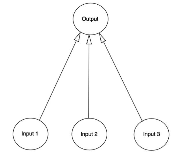
我们可以在计算机上创建神经网络，来对这个过程进行建模，且并不需要模拟分子级的生物复杂性，只要观其大略即可。为了简化起见，我们只模拟一个神经元，含有三个输入和一个输出。

我们将训练这个神经元来解决下面这个问题，前四个样本叫作“训练集”，你能求解出模式吗??处应该是0还是1呢?

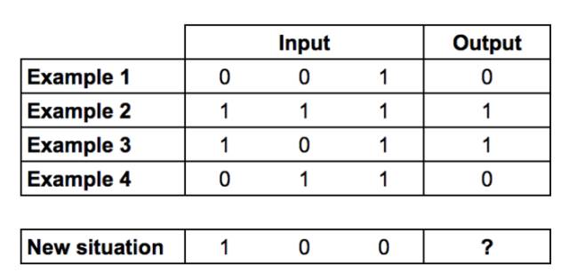
或许已经发现了，输出总是与第一列的输入相等，所以?应该是1。

▍训练过程

问题虽然很简单，但是如何教会神经元来正确的回答这个问题呢?我们要给每个输入赋予一个权重，权重可能为正也可能为负。权重的绝对值，代表了输入对输出的决定权。在开始之前，我们先把权重设为随机数，再开始训练过程：

从训练集样本读取输入，根据权重进行调整，再代入某个特殊的方程计算神经元的输出。

计算误差，也就是神经元的实际输出和训练样本的期望输出之差。

根据误差的方向，微调权重。

重复10000次。

最终神经元的权重会达到训练集的最优值。如果我们让神经元去思考一个新的形势，遵循相同过程，应该会得到一个不错的预测。

▍计算神经元输出的方程

你可能会好奇，计算神经元输出的人“特殊方程”是什么?首先我们取神经元输入的加权总和：

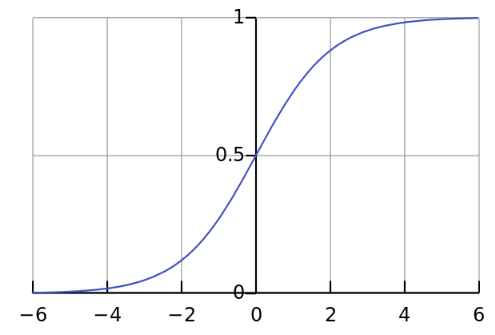
接下来我们进行正规化，将结果限制在0和1之间。这里用到一个很方便的函数，叫Sigmoid函数：

如果绘出图像，Sigmoid函数是S形的曲线：

将第一个公式代入第二个，即得最终的神经元输出方程：

▍调整权重的方程

在训练进程中，我们需要调整权重，但是具体如何调整呢?就要用到“误差加权导数”方程：

为什么是这个方程?首先我们希望调整量与误差量成正比，然后再乘以输入(0-1)。如果输入为0，那么权重就不会被调整。最后乘以Sigmoid曲线的梯度，为便于理解，请考虑：

我们使用Sigmoid曲线计算神经元输出。

如果输出绝对值很大，这就表示该神经元是很确定的(有正反两种可能)。

Sigmoid曲线在绝对值较大处的梯度较小。

如果神经元确信当前权重值是正确的，那么就不需要太大调整。乘以Sigmoid曲线的梯度可以实现。

Sigmoid曲线的梯度可由导数获得：

代入公式可得最终的权重调整方程：

实际上也有其他让神经元学习更快的方程，这里主要是取其相对简单的优势。

▍构建Python代码

尽管我们不直接用神经网络库，但还是要从Python数学库Numpy中导入4种方法：

exp： 自然对常数

array： 创建矩阵

dot：矩阵乘法

random： 随机数

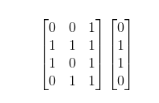
比如我们用array()方法代表训练集：

training_set_inputs = array([[0, 0, 1], [1, 1, 1], [1, 0, 1], [0, 1, 1]])

training_set_outputs = array([[0, 1, 1, 0]]).T

.T函数就是矩阵转置。我想现在可以来看看美化版的源代码了：

最后我还会提出自己的终极思考。源代码中已经添加了注释逐行解释。注意每次迭代我们都一并处理了整个训练集，以下为完整的Python示例：

from numpy import exp, array, random, dot

class NeuralNetwork():

def __init__(self):

# Seed the random number generator, so it generates the same numbers

# every time the program runs.

random.seed(1)

# We model a single neuron, with 3 input connections and 1 output connection.

# We assign random weights to a 3 x 1 matrix, with values in the range -1 to 1

# and mean 0.

self.synaptic_weights = 2 * random.random((3, 1)) - 1

# The Sigmoid function, which describes an S shaped curve.

# We pass the weighted sum of the inputs through this function to

# normalise them between 0 and 1.

def __sigmoid(self, x):

return 1 / (1 + exp(-x))

# The derivative of the Sigmoid function.

# This is the gradient of the Sigmoid curve.

# It indicates how confident we are about the existing weight.

def __sigmoid_derivative(self, x):

return x * (1 - x)

# We train the neural network through a process of trial and error.

# Adjusting the synaptic weights each time.

def train(self, training_set_inputs, training_set_outputs, umber_of_training_iterations):

for iteration in xrange(number_of_training_iterations):

# Pass the training set through our neural network (a single neuron).

output = self.think(training_set_inputs)

# Calculate the error (The difference between the desired output

# and the predicted output).

error = training_set_outputs - output

# Multiply the error by the input and again by the gradient of the Sigmoid curve.

# This means less confident weights are adjusted more.

# This means inputs, which are zero, do not cause changes to the weights.

adjustment = dot(training_set_inputs.T, error * self.__sigmoid_derivative(output))

# Adjust the weights.

self.synaptic_weights += adjustment

# The neural network thinks.

def think(self, inputs):

# Pass inputs through our neural network (our single neuron).

return self.__sigmoid(dot(inputs, self.synaptic_weights))

if __name__ == "__main__":

#Intialise a single neuron neural network.

neural_network = NeuralNetwork()

print "Random starting synaptic weights: "

print neural_network.synaptic_weights

# The training set. We have 4 examples, each consisting of 3 input values

# and 1 output value.

training_set_inputs = array([[0, 0, 1], [1, 1, 1], [1, 0, 1], [0, 1, 1]])

training_set_outputs = array([[0, 1, 1, 0]]).T

# Train the neural network using a training set.

# Do it 10,000 times and make small adjustments each time.

neural_network.train(training_set_inputs, training_set_outputs, 10000)

print "New synaptic weights after training: "

print neural_network.synaptic_weights

# Test the neural network with a new situation.

print "Considering new situation [1, 0, 0] -> ?: "

print neural_network.think(array([1, 0, 0]))

▍结果

Random starting synaptic weights:

[[-0.16595599]

[ 0.44064899]

[-0.99977125]]

New synaptic weights after training:

[[ 9.67299303]

[-0.2078435 ]

[-4.62963669]]

Considering new situation [1, 0, 0] -> ?:

[ 0.99993704]

我们做到了!我们使用Python构建了一个简单的神经网络!

首先，神经网络分配自身随机权重，然后使用训练集训练自己。然后考虑一个新的情况[1，0，0]并预测0.99993704。正确的答案是1.所以非常接近!

传统的电脑程式通常无法学习。神经网络令人惊奇的是可以自学习，适应和应对新情况。

github：https://github.com/miloharper/simple-neural-network