什么是监督学习？

在监督学习中，我们首先要导入包含训练特征和目标特征的数据集。监督式学习算法会学习训练样本与其相关的目标变量之间的关系，并应用学到的关系对全新输入（无目标特征）进行分类。

为了说明如何监督学习的原理，让我们看一个根据学生学习的时间来预测学生的成绩的例子。

公式：

Y = f（X）+ C

在这里：

F表示学生为考试准备的小时数和分数之间的关系
X是输入（他睡觉的小时数）
Y是输出（标记在考试中学生的得分）
C是随机误差

监督学习算法的最终目标是以最大精度来预测给定新输入X所对应的Y.有很多种方法可以实现监督学习; 我们在这里讨论一些最常用的方法。

根据给定的数据集，机器学习问题分为两类：分类和回归。如果给定数据同时具有输入（训练）值和输出（目标）值，那么这是一个分类问题。如果数据集具有连续的没有任何目标标记的特征数值，那么它属于回归问题。

分类：输出标签：这个是猫还是狗？

回归：这个房子卖多少钱？

分类

以想要分析乳腺癌的数据的医学研究人员为例。目标是预测患者应接受三种治疗方法中的哪一种。这种数据分析任务被称为分类，在这个分类中，模型或分类器被构造来预测类标签，例如“治疗a”、“治疗B”或“治疗c”。

分类是预测问题，预测离散和无序的分类的类标签。这一过程，由学习步骤和分类步骤两部分组成。

分类中方法

最常用的分类算法：

1.KNN算法（K-Nearest Neighbo）

2.决策树

3.朴素贝叶斯

4. 支持向量机

在学习步骤中，分类模型通过分析训练集来建立分类器。在分类步骤中，预测给定数据的类标签。在分析中，数据集元组及其关联的类标签分为训练集和测试集。构成训练集的各个元组从随机抽样的数据集中进行分析。剩下的元组形成测试集，并且独立于训练元组，也就是说它们不会用来构建分类器。

测试集用于估计分类器预测的准确性。分类器的准确性是指由分类器正确分类的测试元组的百分比。为了达到更好的准确性，最好测试不同的算法，并在每个算法中尝试不同的参数。最好通过交叉验证进行选择。

想要为某个问题选择合适的算法，对于不同的算法，精度、训练时间、线性度、参数个数和特殊情况等参数都需要考虑。

在IRIS数据集上使用Scikit-Learn实现KNN，根据给定的输入对花进行分类。

第一步，为了应用我们的机器学习算法，我们需要了解和探索给定的数据集。在这个例子中，我们使用从scikit-learn包导入的IRIS数据集（鸢尾花数据集）。现在让我们来编码并探索IRIS数据集。

确保你的机器上已经安装了Python。然后使用PIP安装以下软件包：

在这段代码中，我们使用pandas中的几种方法了解了IRIS数据集的属性。

输出：

Scikit-learn中的KNN

如果一个算法只是简单地存储训练集的元组并等待给出测试元组，那么他就是一个惰性学习法。只有当它看到测试元组时才会执行泛化，基于它与训练元组的相似度对元组进行分类。

KNN是一个惰性学习法。

KNN基于类比学习，比较出给定的测试元组与训练元组的相似度。训练元组由n个特征描述。每个元组代表一个n维空间中的一个点。这样，所有的训练元组都存储在n维模式空间中。当给定未知元组时，KNN分类器在模式空间中搜索最接近未知元组的k个训练元组。这k个训练元组是未知元组的k个“最近邻（nearest neighbor）”。

贴近度（Closeness）由关于距离的度量定义（例如欧几里得度量）。一个好的K值要通过实验确定。

在这段代码中，我们从sklearn中导入KNN分类器，并将其应用到我们的输入数据，对花进行分类。

输出：

在这里：

0对应的Versicolor
1对应的Virginica
2对应Setosa

（注：都是鸢尾花的种类）

基于给定的输入，机器使用KNN预测两个花都是Versicolor。

IRIS数据集分类直观图：

回归

回归通常被用于确定两个或多个变量之间的关系。例如，根据给定的输入数据X，你必须预测一个人的收入。

在回归里，目标变量是指我们想要预测的未知变量，连续意味着Y可以承担的值没有缺口（或者说间断点）。

预测收入是一个典型的回归问题。你的输入数据包含所有可以预测收入的信息（即特征）。比如他的工作时间，教育经历，职位和居住地。

回归模型

一些常用的回归模型是：

• 线性回归

• Logistic回归

• 多项式回归

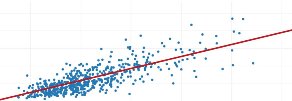
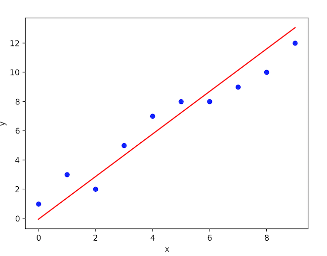
线性回归使用最佳拟合直线（也称回归线）建立因变量（Y）和一个或多个自变量（X）之间的关系。

用公式表示：

h（xi）=βo+β1* xi + e

其中βo是截距，β1是线的斜率，e是误差项。

线性回归

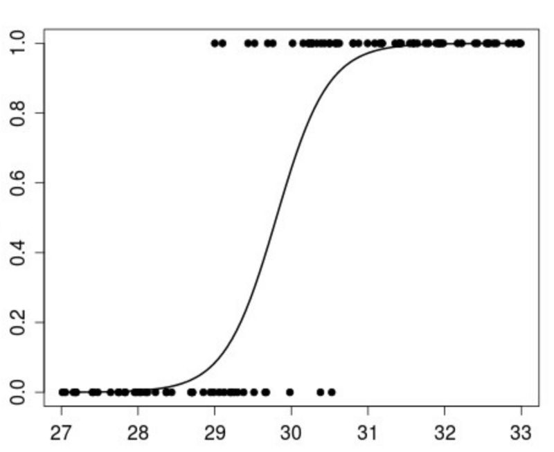
Logistic回归是一种算法，可以在响应变量是分类（categorical）时使用。Logistic回归的思想是找出特征和特定结果的概率之间的关系。

用公式表示为：

p（X）=βo+β1* X

p（x）= p（y = 1 | x）

Logistic回归

多项式回归是一种回归分析方法，其中自变量x和因变量y之间的关系被建模为x中的一个n次多项式。

解决线性回归问题：

我们有数据集X和相应的目标值Y，我们使用最小二乘法来学习一个线性模型，我们可以使用这个线性模型来预测一个新的y，给出一个未知的x，它的误差越小越好。

将给定的数据被分成训练数据集和测试数据集。训练集具有标签（加载特征），所以算法可以从这些标签的例子中学习。测试集没有任何标签，也就是说，你还不知道这个值，试图去预测。

我们将拿出一个特征进行训练，并应用线性回归方法来拟合训练数据，然后使用测试数据集预测输出。

线性回归在scikit-learn中的实现：

输出：

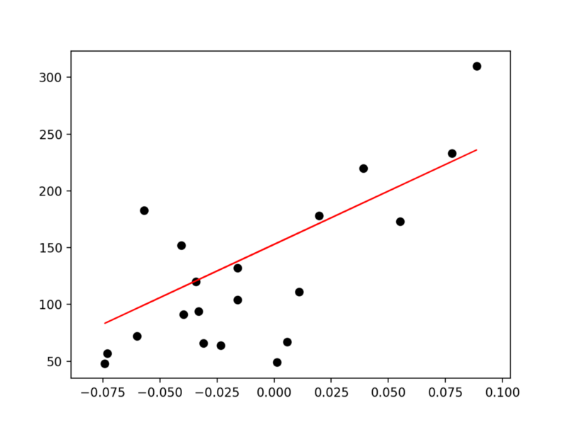
预测diabetes_X_test和diabetes_y_pred之间的图在线性方程上连续。

• 代码：https://github.com/vihar/supervised-learning-with-python